
Understanding Historian Deadband and the Hidden Slow Drift Problem
A data historian records how an industrial process behaves over time, but it does not record everything. The deadband is the threshold a historian uses to skip value changes it considers insignificant: when a measurement moves less than the threshold, the historian treats the change as noise and does not store a new value. That keeps storage and communication load down.
The filter works well for fast, noisy signals. It also creates a failure mode that is easy to miss. Slow drift — a sensor or process variable moving gradually over hours, days, or weeks — usually advances in steps smaller than a wide deadband. Each step stays below the threshold, so the historian writes nothing, and a real trend never makes it into the stored record.
Set the deadband too wide and slow drift is filtered out of the record. The archive can look perfectly stable while the process underneath is moving. That gap between what happened and what was kept is the subject here.
The practical way to reveal the gap is to put raw and archived trends side by side. Raw trends come from the raw scan or high-resolution layer, where every collected sample is kept. Archived trends come from the historian after deadband filtering has reshaped the data. Plotted together, the two diverge: the raw line climbs or falls steadily while the archived line stays flat or steps only now and then.
The comparison matters to anyone who works from the archive. Historians need to document what it actually contains and where filtering has shaped it. Analysts can reach the wrong conclusion when archived trends are their only evidence. Engineers may miss a degrading sensor or a slow process shift that has not yet crossed an alarm. Researchers need a faithful long-term series before they can trust their results. Knowing how a wide deadband hides slow drift is the first step toward retention and filtering policies that preserve the signal, not just the storage.
How Deadband Compression Works in a Process Historian
A process historian collects far more samples than it can economically store or a person can usefully review. Tags update several times a second across thousands of points, so a database that wrote every reading would fill up with noise. Deadband compression decides, tag by tag, which incoming values are worth keeping: the historian stores a value only when it moves beyond a tolerance the engineer sets.
The comparison loop. When a new sample arrives, the historian compares it against the last value it stored — not the previous sample, but the most recent entry in the archive. It measures the difference and tests it against the configured threshold. If the change is small, the sample is discarded. If it exceeds the threshold, the value is written and becomes the new reference point. Because the reference moves only when data is stored, the logic behaves like a running filter over the live stream, and long stretches of near-steady behavior collapse into a single archived entry.
Absolute deadband. An absolute deadband is a fixed number in the tag’s own engineering units — say, 0.5 degrees for a temperature point. The tolerance stays the same no matter how large the tag’s range is. That makes it predictable and easy to reason about, and it suits tags whose natural variation is well understood.
Percentage-of-span deadband. A percentage-of-span deadband scales the threshold to the tag’s configured range. If the span runs from 0 to 100 and the deadband is set to 1 percent, the effective tolerance is 1 unit. A larger range means a coarser filter. That keeps compression consistent across tags with very different physical scales, but it can also hide small movements in a wide-range signal.
| Deadband type | Threshold defined as | Tolerance behavior |
|---|---|---|
| Absolute | Fixed value in engineering units | Constant across the tag’s range |
| Percentage of span | Fraction of the configured range | Grows as the range grows |
Exception-based data storage. Exception reporting applies the same principle to time: instead of recording on a fixed schedule, the system stores a record only when a defined exception occurs — a change beyond the deadband. Those stored points are what trend displays and reports draw from. The discarded raw data is gone once it passes through the comparison.
Why it matters. Compression only works when the deadband matches the dynamics of each tag. Set it too tight and the historian stores redundant points. Set it too wide and slow drift slips under the threshold, leaving an archive that looks flat while the raw data keeps moving.
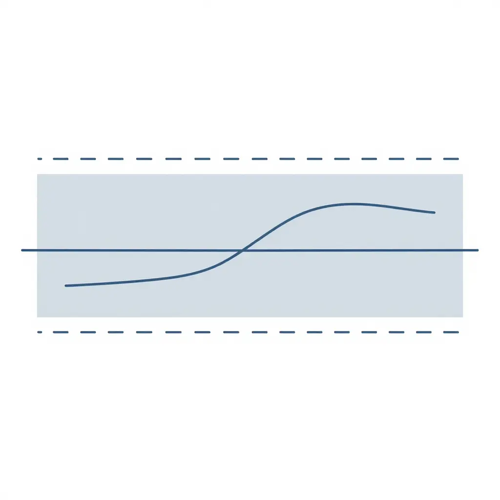
The schematic shows how a wide deadband suppresses visible change. The horizontal line is the steady recorded value; the two dashed lines mark the upper and lower deadband boundaries. The drifting signal stays inside that band for most of its journey, so the archive logs no update at all. The drift stays hidden until the signal finally crosses a boundary, and then the trend appears to jump.
Why an Over-Wide Deadband Hides Slow Drift
A process historian does not archive every measurement it reads. To cut storage demand and reject signal noise, it records a new value only when the incoming signal differs from the last stored value by more than a configured amount, the deadband. Raise that threshold too high — a wide deadband — and the archive stops being a continuous record and becomes a series of coarse snapshots.
The chain is simple. The deadband sets the smallest change that triggers a new archive entry. A wide deadband puts that trigger well above the small movements a sensor makes on each scan. During slow drift, the measured value creeps up or down in tiny, steady increments — fractions of a unit per day. No single increment exceeds the threshold. The change never crosses the trigger, so the historian has no reason to write a new record, and the value that would have been captured is discarded. The process keeps changing; the stored number does not.
That is how slow drift accumulates without a trace. A temperature, pressure, current, or flow reading wanders away from its original operating point, and nothing in the logging system flags it. Only when the accumulated deviation grows large enough to exceed the deadband does the historian log a new entry — one that has jumped to reflect a change that actually built up over weeks or months. The archive then shows a sudden step instead of a gentle slope, hiding the true rate and duration of the movement.
The contrast between the two views is the core of the problem:
| Trend View | What It Captures | What It Hides |
|---|---|---|
| Raw trend | Every incremental movement, the true slope, direction, and elapsed time of the drift | Signal noise and scan-level jitter |
| Archived trend | Only changes exceeding the deadband threshold | Gradual low-magnitude change, the genuine onset and rate of drift |
A raw trend plotted straight from the live signal or a high-resolution capture shows every incremental movement: the gradual slope, the direction of travel, and how long the drift has been developing. The archived trend, filtered through the wide deadband, hides that slope. It reads as a flat line punctuated by occasional steps, as if the process were stable right up until the moment it changed.
A flat archived trend is not proof of stability. It may only prove that the deadband was too wide to record what was happening. Decisions about maintenance, calibration, or process optimization made from the archived trend alone can rest on false assumptions. Comparing the raw trend against the archived trend restores the missing information: the slow drift the archive suppressed becomes visible, and the real rate of change can be measured instead of inferred.
Deadband Width vs. Drift Sensitivity
The table below maps deadband settings to what they do in practice, both to the storage footprint and to the ability to catch slow-moving changes. It makes the trade-off plain: as deadbands widen, archived data volume shrinks, and drift visibility goes with it.
| Deadband Width | Threshold Required to Trigger Storage | Detection Sensitivity to Slow Drift | Archived Data Volume | Risk of Concealed Drift |
|---|---|---|---|---|
| 0.1% (very narrow) | Nearly any measurable change is captured | Extremely high – even the gentlest ramp is logged | Very large; close to raw signal | Very low |
| 0.5% (narrow) | Small changes relative to range are captured | High – gradual trends remain fully visible | Large | Low |
| 1.0% (moderate) | Change must exceed ~1% of span | Medium – slow drifts stay visible but soften | Moderate | Moderate |
| 2.0% (wide) | Change must exceed ~2% of span | Reduced – slow drift is partially masked | Small | Elevated |
| 5.0% (very wide) | Change must exceed ~5% of span | Low – slow drift often never fires | Very small | High |
| 10.0% (extremely wide) | Change must exceed ~10% of span | Minimal – only large jumps trigger a record | Tiny; sparse snapshots | Severe |
Reading the Trade-Off
The pattern is consistent. A wider deadband buys a smaller archive by raising the threshold a value must cross before anything is written. A sensor creeping upward can sit below that threshold for hours — or days — producing a flat, stable archived line while the raw signal drifts away from it. That is why the Risk of Concealed Drift climbs as Archived Data Volume falls. Narrow deadbands keep fidelity and cost storage; wide deadbands keep storage and cost truth. When you are diagnosing slow process changes, cross-check the archived trend against a raw or short-term capture before you trust a suspiciously flat line.
Methodology: Comparing Raw and Archived Trends to Expose Hidden Drift
A wide deadband suppresses low-amplitude variation at the compression stage, so the stored history can look flat while the process walks away from its setpoint. The steps below compare the uncompressed signal against what the historian retained, and make any drift the deadband concealed measurable.
1. Define the comparison window and tag set. Pick a contiguous time range long enough to capture slow movement — several shifts or days, not minutes. Choose the process tags of interest and record their sampling intervals, engineering units, and the deadband configuration in force during the period. Writing these parameters down first means a later discrepancy can be attributed to compression and not to a configuration change.
2. Perform the raw data export. Pull the highest-resolution values available from the source layer — the controller, edge device, or full-fidelity buffer — rather than from the compressed history. This raw data export has to preserve the original native timestamps and the full decimal precision of each reading. Store it as an immutable file so the reference series is never overwritten during analysis.
3. Export the archived trend. Retrieve the same tags over the identical window from the historian. This archived trend is exactly what downstream users, reports, and dashboards consume, so it is the honest record of the organization’s view of the past. Keep the archived export separate and clearly labeled.
4. Align both series on a common time axis. Sampling rates and interpolation policies usually differ, so complete a timestamp alignment pass before any comparison. Resample both series onto a shared, uniform interval (for example, one minute), decide explicitly whether to interpolate or forward-fill, and convert both to identical time zones and units. Misaligned axes produce phantom divergence, so verify that the first and last aligned points correspond to the same physical event.
5. Compute the divergence. Subtract the archived value from the raw value at each aligned point to get a residual series. Report the residual magnitude, the signed error, the cumulative sum of residuals, and the time the residual first exceeds a chosen threshold. A slow, monotonic residual is the signature of hidden drift; a random residual is simply quantization noise.
6. Interpret for drift detection. Sustained non-zero residuals are evidence that the deadband is too wide. Quantify the slope of the residual against time to estimate the rate at which the archived value falls behind reality, then compare that slope against the process tolerance.
7. Validate and document. Confirm the finding on an independent window, note the deadband value under test, and record the recommended tighter setting. Repeating this workflow establishes a defensible, auditable basis for tuning compression parameters without sacrificing long-term data quality.
How a Wide Deadband Flattens Slow Drift
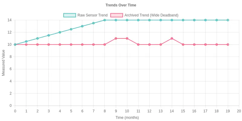
The chart plots two series on a shared time axis. The raw sensor trend (teal line) climbs smoothly from roughly 10 to 14 over the 20-month window, showing the gentle, continuous upward drift that is actually happening in the measurement. The archived trend (pink line) tells a very different story: the historian’s deadband was set too wide, so the archive ignores every small change and nudges its stored value only when movement finally exceeds the threshold. The result is a nearly flat, stepped line that hides the drift almost entirely.
Reading the Divergence
The gap between the two lines is the heart of the problem. A deadband exists to reduce storage noise, but when it is calibrated too aggressively it stops recording the slow, low-amplitude changes that long-term analysis depends on.
| Signal | Behavior | What It Reveals |
|---|---|---|
| Raw sensor trend | Steady upward climb (10 to 14) | The true, continuous direction of drift |
| Archived trend | Flat, occasional small steps | Drift suppressed by an oversized deadband |
Why It Matters
- Slow drift accumulates. A change of a few units per year looks harmless on its own, but over many years it distorts calibration records, environmental monitoring, and equipment history.
- The archive becomes misleading. Rely on archived values alone and you may conclude that nothing changed, while the raw data says otherwise.
- Trend analysis breaks down. Stepped data hides slope and rate of change, defeating the purpose of a historian in the first place.
Tune the deadband to the amplitude of the slowest change you need to preserve. If the archived line looks suspiciously flat while the raw line is clearly drifting, the deadband is too wide.
Detected Drift Events vs. Deadband Width
The bar chart below compares how many drift events a historian detects as the deadband width grows from very narrow to very wide. Each bar is a different deadband setting; its height is the number of drift events the archive actually captures.
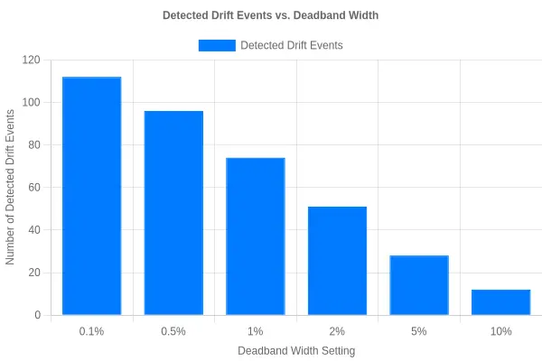
The downward trend is the whole story. A tight 0.1% deadband surfaces 112 drift events, while a wide 10% deadband catches only 12. By the time the deadband reaches 5% or 10%, the slow, gradual drift that usually precedes a real equipment failure simply stops registering as a distinct event. The data hasn’t changed; the filter has just decided that most of the movement isn’t worth recording.
Related Resources
The pages below are unrelated to deadband configuration and cover other topics from elsewhere on this site.
- A guide to the top 10 dirt bike wraps.
- An overview of custom dirt bike graphics and the customization workflow.
- A reference on dirt bike graphics kits.
- Applied configuration examples using custom graphics for dirt bikes.
- A roundup of top 10 dirt bike graphics tricks.
FAQ: Historian Deadband and Drift Detection
What is a historian deadband?
A historian deadband is a threshold that tells the data collection system to store a new value only when it differs from the last archived value by more than a set amount. If a reading stays within that band, the historian skips it and keeps the previous sample. That cuts storage and network load by filtering out tiny fluctuations. The deadband can be set in absolute engineering units or as a percentage of span.
Why does a wide deadband hide slow drift?
Slow drift unfolds over hours, days, or weeks, so the movement between two adjacent scans is very small. A wide deadband means those increments never exceed the threshold, and the historian keeps recording the same stale value. The signal can wander far from its true position while the archive shows a flat line. By the time the accumulated change crosses the deadband, the chance to catch and correct the trend early is gone.
How do raw trends differ from archived trends?
Raw trends show every value the controller or sensor produces at its full scan rate, with no filtering. Archived trends show only the values the historian stored after the deadband logic ran. A raw trend therefore reveals gradual movement, noise, and micro-fluctuations that an archived trend smooths or drops. Put the two side by side and you can see what the deadband is discarding.
How can I test whether my deadband is too wide?
Record a raw trend from the source at the full scan rate and put it beside the archived trend for the same period. If the archived line is flat or stepping while the raw line slopes gradually, the deadband is hiding slow drift. You can also inject a known slow ramp into a test point and see whether the historian captures its progress. If the ramp stays invisible until it exceeds the threshold, the setting is too aggressive.
What is a reasonable starting point for deadband tuning?
A common starting point is a deadband of roughly 0.5 to 1 percent of the instrument’s measurement span, adjusted for the process dynamics. Fast or safety-critical loops need narrower bands, while slow, noisy variables can tolerate wider ones. Validate any setting by comparing raw trends and archived trends over several days. Always favor drift visibility over storage savings when the variable matters to quality or safety.
Balancing Deadband and Drift Visibility
A deadband set too wide quietly trades accuracy for storage. A generous threshold reduces archive volume and lightens the load on the historian, but it also conceals slow drift — a process value migrating gradually, never tripping an alarm, steadily eroding efficiency, safety margins, and product quality. Compression hides what it judges insignificant, and slow drift falls into that category until it becomes a problem.
The remedy is comparison. Put raw trends beside archived trends over the same window and the gap between them shows what the deadband discarded. The archived line looks flat and stable; the raw line shows the climb or creep the threshold swallowed. That check turns an invisible risk into an obvious one.
A Practical Takeaway for Every Role
For historians and data analysts the habit is the same: do not trust a trend on its own. Pull the raw data and overlay it against the archived version before drawing conclusions.
- Historians should document the deadband setting applied to each tag. The configuration is part of the record and shapes every downstream reading.
- Data analysts should treat archived trends as a summary, not a source of truth, and check anomalies against uncompressed data.
- Engineers should audit deadband settings on a schedule, tightening them where trend fidelity matters more than storage savings.
- Researchers should keep raw data accessible so results stay reproducible.
Auditing deadband settings only works if the raw access is still there. Compression is useful when you can see past it. Keep the raw stream available, review the thresholds that thin it, and make the comparison between raw and archived trends the standard safeguard against drift that would otherwise stay hidden.